User Guide#

This user guide shows you different examples of how to use decent-bench.

Installation#

pip install decent-bench

Sunny case#

Benchmark algorithms on a regression problem without any communication constraints, using only default settings.

Generally benchmark execution involves three steps:

Run algorithms on a BenchmarkProblem object and get results in a BenchmarkResult object.
Compute metrics from the benchmark results, which returns a MetricResult object.
Display the computed metrics in tables and plots.

Note:: When running benchmarks, be sure to guard the execution code with if __name__ == "__main__": to avoid issues with multiprocessing on some platforms (e.g., Windows). This is a common Python practice to ensure that the benchmark code only runs when the script is executed directly, and not when it is imported as a module or when worker processes are spawned for multiprocessing. If you forget to include this guard and you are using multiprocessing, i.e. with max_processes > 1 in benchmark(), you may encounter errors or unexpected behavior due to the way multiprocessing works on different platforms.

The following is a working example. The remainder of the user guide will be updated soon.

from decent_bench.agents import Agent
from decent_bench import benchmark
from decent_bench.metrics import runtime_library
from decent_bench.utils.checkpoint_manager import CheckpointManager
from decent_bench.distributed_algorithms import DGD, ATC
from decent_bench.networks import P2PNetwork
from decent_bench.benchmark import create_quadratic_problem

import networkx as nx

if __name__ == "__main__":
    ## problem definition
    n_agents = 10

    costs, x_optimal = create_quadratic_problem(10, n_agents)

    agents = [Agent(cost) for i, cost in enumerate(costs)]
    graph = nx.complete_graph(n_agents)

    net = P2PNetwork(
        graph=graph,
        agents=agents,
    )

    bp = benchmark.BenchmarkProblem(net, x_optimal)

    ## benchmarking
    cm = CheckpointManager(checkpoint_dir="results/benchmark_1", checkpoint_step=100, keep_n_checkpoints=2)

    num_iter = 1000
    step = 0.001

    res = benchmark.benchmark(algorithms=[
            DGD(iterations=num_iter, step_size=step),
            ATC(iterations=num_iter, step_size=step),
        ],
        benchmark_problem=bp,
        checkpoint_manager=cm,
        n_trials=1,
        )

    metr = benchmark.compute_metrics(res, checkpoint_manager=cm)

    benchmark.display_metrics(metr, checkpoint_manager=cm)

Benchmark executions will have outputs like these:

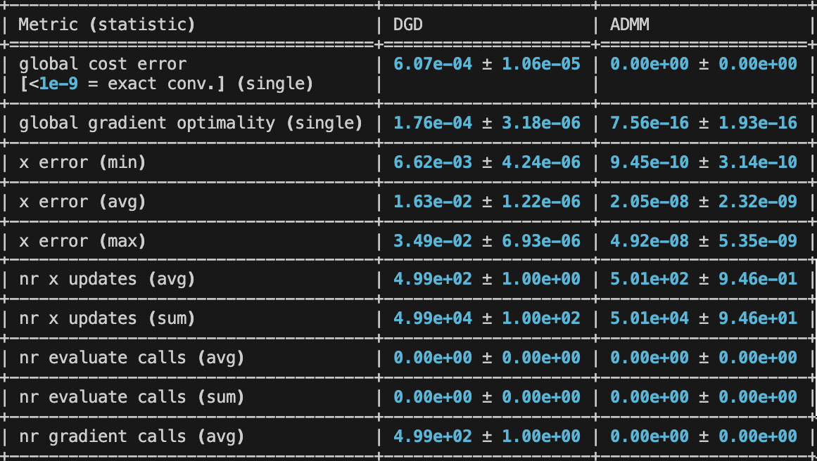
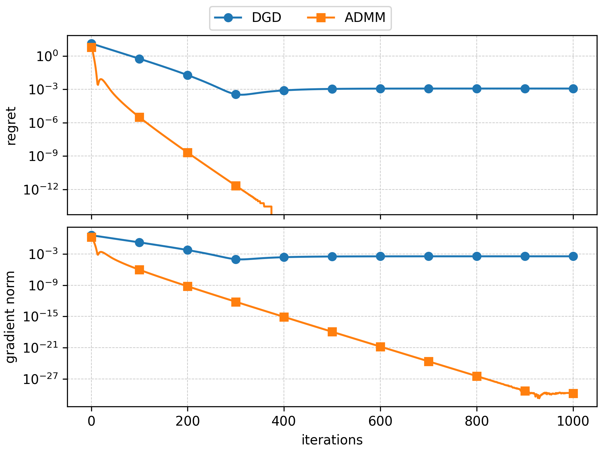
The user guide from here on is outdated; it will be updated soon.

Available algorithms#

Note: algorithms are slightly modified with respect to the corresponding papers to ensure that they work in a broader range of conditions (asynchorny/partial participation, loss of communications, etc) than the original papers.

Peer-to-peer#

ADMM [dual method, ADMM]
ATG [gradient-tracking, dual method, ADMM]
ATC [gradient-based]
ATC_Tracking [gradient-tracking]
AugDGM [gradient-tracking]
DGD [gradient-based]
DLM [ADMM, gradient-based]
DiNNO [gradient-based]
ED [gradient-tracking]
EXTRA [gradient-tracking]
GT_SAGA [gradient-tracking]
GT_SARAH [gradient-tracking]
GT_VR [gradient-tracking]
KGT [gradient-based]
LED [gradient-based]
LT_ADMM [gradient-based, dual method, ADMM]
LT_ADMM_VR [gradient-based, dual method, ADMM, variance-reduction]
NIDS [gradient-tracking]
ProxSkip [gradient-based]
SimpleGT [gradient-tracking]
WangElia [gradient-tracking]

Federated#

FedAvg performs local client gradient steps from the broadcast server model and then replaces the server model with the uniform average of the received final client models.

FedProx extends FedAvg with a proximal coefficient penalty. In the FedProx equations, the symbol \(\mu\) is used for this coefficient, and the corresponding argument is penalty. Setting penalty=0 reduces FedProx to FedAvg.

FedAdagrad, FedYogi, and FedAdam form the built-in FedOpt family. They keep the same client-side local SGD structure as FedAvg, but each client uploads its model delta to the server and the server applies an adaptive optimizer update instead of plain averaging to the next global iterate.

FedNova supports the plain Local-SGD FedNova update together with optional local momentum, proximal local updates, and server momentum. Clients accumulate their local updates together with the FedNova normalization coefficient and upload them to the server in two separate transmissions before the server applies the aggregated update. If none of the first-phase normalizer uploads are received in a round, that round is skipped without updating the server model. The num_local_steps argument can be either a single integer for homogeneous local work or a per-client mapping for heterogeneous local step counts.

FedLT implements Federated Local Training with cost-driven local gradients. Its local_solver option supports "gd", "nesterov", and "adam" local updates. Solver-specific hyperparameters are passed through solver_args. If solver_args is omitted or left empty, solver-specific defaults are used: "nesterov" uses momentum=0.9, "adam" uses beta1=0.9, beta2=0.999, and epsilon=1e-8, and "gd" uses no additional solver arguments. EmpiricalRiskCost objects use their default mini-batch gradient behavior, so gradient-based local solvers use mini-batches, while generic Cost objects use full gradients. Fed-LT compression and Fed-PLT-style noisy-message experiments are configured through FedNetwork message_compression and message_noise schemes rather than algorithm arguments.

SCAFFOLD implements stochastic controlled averaging with a server control variate and one client control variate per client. Selected clients run local steps corrected by the difference between the server and client control variates, then upload both their model delta and control-variate delta. The server applies the averaged model delta with server_step_size and updates its control variate using the participation fraction.

FedPD implements the FedPD primal-dual update. Clients keep persistent local primal variables, dual variables, and centre candidates. Each round uses num_local_steps local gradient steps on the augmented Lagrangian, with step_size controlling the local learning rate and penalty controlling the FedPD quadratic penalty/dual-update parameter. The skip_probability argument controls the paper’s optional communication skipping: 0 aggregates every round and 1 always keeps local centre candidates without server aggregation. Like FedNova, num_local_steps can be either a single integer or a per-client mapping. FedPD always uses all active clients; partial participation is not supported.

FedDyn implements Federated Dynamic Regularization. Clients keep a persistent dynamic state g and the server keeps an auxiliary vector h. Selected clients run num_local_steps local gradient steps on the dynamic-regularized local objective using step_size as the local learning rate and penalty as the regularization coefficient. In the FedDyn equations, the symbol \(\alpha\) denotes this regularization, and the corresponding argument is penalty.

Federated aggregation#

For the built-in federated algorithms, aggregation affects only how client updates are combined at the server. It does not change the optimization objective itself. If you want to optimize a weighted objective, scale the client costs in the problem definition instead of relying on aggregation.

FedAvg and FedProx use uniform averaging over the selected clients.

FedAdagrad, FedYogi, and FedAdam also average client model deltas uniformly over the selected clients before applying their server-side adaptive optimizer.

FedNova uses data-proportional client weights over the received uploads in the round, and it does not average final client models directly when local step counts differ. Instead, it aggregates the client cumulative SGD updates using the FedNova rescaling factor and applies the resulting descent step at the server. With the default flags, this is the plain no-momentum FedNova variant. Enabling use_momentum, use_prox, or use_server_momentum extends the local and server updates to the corresponding FedNova variants controlled by momentum, penalty, and server_momentum. In the FedNova equations, symbols \(\beta\), \(\mu\), and \(\gamma\) map to those arguments respectively. Plain FedNova matches FedAvg only when the participating clients use the same number of local steps and FedNova and FedAvg both use data-proportional aggregation weights.

FedPD aggregates received centre candidates uniformly when communication is not skipped.

FedDyn averages the received selected-client models uniformly, so the local-model average is scaled by the number of received selected clients. The next server model also includes the FedDyn dynamic correction from the server auxiliary vector h. The h update uses only received client models and scales their model deltas by the total number of clients.

Scaffold matches the standard SCAFFOLD algorithm and always uses uniform averaging over the selected clients.

Client selection#

Federated algorithms accept a selection_scheme argument. The scheme receives the active clients for the current round and returns the subset that should receive the server broadcast.

UniformSelection samples active clients uniformly without replacement. This is the default for the built-in federated algorithms.

DataSizeSelection samples active clients without replacement with probabilities proportional to client data size. This is useful when local dataset sizes are imbalanced and you want larger clients to have more participation opportunities. The scheme reads data size from EmpiricalRiskCost.n_samples, so it requires clients to use empirical-risk costs.

FairSelection prioritizes clients with fewer past selections. This is useful when availability or random sampling can repeatedly skip some clients and you want selection opportunities to remain balanced across rounds.

HighLossSelection evaluates client losses at each client’s current x and selects the clients with highest loss.

from decent_bench.algorithms.federated import FedAvg
from decent_bench.schemes import DataSizeSelection

algorithm = FedAvg(
    iterations=100,
    step_size=0.01,
    selection_scheme=DataSizeSelection(fraction_selected_clients=0.1),
)

Available costs#

Regression#

LinearRegressionCost [empirical-risk]
PyTorchCost [classification, empirical-risk]

Classification#

LogisticRegressionCost [empirical-risk]
PyTorchCost [regression, empirical-risk]

PyTorchCost regularization#

When combining PyTorchCost with one of the built-in regularizers, instantiate the regularizer with the same framework and device as the empirical cost:

from decent_bench.costs import L2RegularizerCost
from decent_bench.utils.types import SupportedFrameworks

reg = L2RegularizerCost(
    shape=cost.shape,
    framework=SupportedFrameworks.PYTORCH,
    device=cost.device,
)
objective = cost + reg

This preserves compatibility with the PyTorch empirical objective and keeps the resulting objective in the empirical, batch-compatible abstraction. It is convenient for composition, but it is not necessarily the most efficient option compared with native framework-specific regularization.

Execution settings#

Configure settings for metrics, trials, logging, and multiprocessing.

from logging import DEBUG
import numpy as np

from decent_bench.metrics import utils
from decent_bench import benchmark
from decent_bench.costs import LinearRegressionCost
from decent_bench.distributed_algorithms import ADMM, DGD
from decent_bench.metrics import ComputationalCost
from decent_bench.metrics.metric_library import GradientCalls, Regret
from decent_bench.metrics.runtime_library import RuntimeLoss, RuntimeRegret

if __name__ == "__main__":
    regret = Regret(x_log=False, y_log=True)
    gradient_calls = GradientCalls([min, np.average, max, sum])

    benchmark_result = benchmark.benchmark(
        algorithms=[DGD(iterations=1000, step_size=0.01), ADMM(iterations=1000, penalty=10, relaxation=0.3)],
        benchmark_problem=benchmark.create_regression_problem(LinearRegressionCost),
        n_trials=10,
        max_processes=1,
        progress_step=200,
        show_speed=True,
        log_level=DEBUG,
        runtime_metrics=[
            RuntimeLoss(update_interval=100, save_path="results"), # Runtime plots are saved to "results" directory after execution
            RuntimeRegret(update_interval=100, save_path="results"),
        ],
    )

    metrics_result = benchmark.compute_metrics(
        benchmark_result,
        table_metrics=[regret, gradient_calls],
        plot_metrics=[regret],
        log_level=DEBUG,
    )

    benchmark.display_metrics(
        metrics_result,
        table_metrics=[gradient_calls], # Can modify which metrics are displayed, cannot add new metrics that were not computed
        plot_metrics=[], # Disable plot metrics to only show tables
        table_fmt="latex",
        plot_grid=False,
        individual_plots=False,
        computational_cost=ComputationalCost(proximal=2.0, communication=0.1),
        compare_iterations_and_computational_cost=True,
        save_path="results", # Save tables and plots to the "results" directory
    )

For plot metrics some special options are available which change how they are displayed. If you set individual_plots = True then each plot metric will be displayed in its own separate figure, otherwise groups of up to 3 plot metrics will be displayed together in the same figure as subplots. If you set compare_iterations_and_computational_cost = True, then an additional column of subplots will be added to each figure comparing iterations and computational cost, which can be useful to understand the trade-off between faster convergence and higher computational cost for different algorithms.

Interpreting Metric Warnings#

Warnings during metric computation and display are expected in some scenarios, especially when algorithms diverge or when metric prerequisites are not provided.

Unavailable metrics#

Some metrics require additional problem information.

regret and x error require problem.x_optimal.
accuracy, mse, precision, and recall require problem.test_data and
agents with EmpiricalRiskCost.
accuracy, precision, and recall additionally require integer-valued targets.
Federated server metrics such as server accuracy and server mse require
FedNetwork and use the explicit server model history.

If these requirements are not met, the metric marks itself unavailable, a warning is given, and is omitted from the final metric lists returned by compute_metrics().

Plot truncation warnings#

Plot metric trajectories are truncated at the first non-finite datapoint (NaN/inf) or first datapoint above the internal plotting threshold used for log-scale stability.

Typical messages include:

Truncating plot computation ... retained K point(s) from M/N trial(s).
Skipping plot computation ... all trials diverged before the first plottable datapoint.

These warnings indicate that divergence was detected and handled gracefully for plotting.

Why tables can show NaN while plots still appear#

Tables and plots summarize different parts of the trajectory:

Table metrics typically use the final iteration.
Plot metrics may retain and display an earlier finite prefix.

So it is expected to see nan ± nan in a table for a metric while still seeing a corresponding curve in the plot.

Benchmark problems#

Configure out-of-the-box regression problems#

Configure communication constraints and other settings for out-of-the-box regression problems.

The agent_state_snapshot_period parameter controls how often metrics are recorded. Setting it to a value greater than 1 (the default) can help reduce overhead for long-running algorithms while still providing enough data points for analysis. This also speeds up metric calulation and plotting, which can be significant for large benchmarks with many iterations and agents.

from decent_bench import benchmark
from decent_bench.costs import LinearRegressionCost
from decent_bench.distributed_algorithms import ADMM, DGD, ED

problem = benchmark.create_regression_problem(
    LinearRegressionCost,
    n_agents=100,
    agent_state_snapshot_period=10, # Record metrics every 10 iterations
    n_neighbors_per_agent=3,
    asynchrony=True,
    compression=True,
    noise=True,
    drops=True,
)

if __name__ == "__main__":
    benchmark_result = benchmark.benchmark(
        algorithms=[
            DGD(iterations=1000, step_size=0.01),
            ED(iterations=1000, step_size=0.01),
            ADMM(iterations=1000, penalty=10, relaxation=0.3),
        ],
        benchmark_problem=problem,
    )
    metrics_result = benchmark.compute_metrics(benchmark_result)
    benchmark.display_metrics(metrics_result)

Modify existing problems#

Change the settings of an already created benchmark problem, for example, the network topology.

import networkx as nx

from decent_bench import benchmark
from decent_bench.costs import LinearRegressionCost
from decent_bench.distributed_algorithms import ADMM, DGD, ED

n_agents = 100
n_neighbors_per_agent = 3

problem = benchmark.create_regression_problem(
    LinearRegressionCost,
    n_agents=n_agents,
    n_neighbors_per_agent=n_neighbors_per_agent,
    asynchrony=True,
    compression=True,
    noise=True,
    drops=True,
)

problem.network_structure = nx.random_regular_graph(n_agents, n_neighbors_per_agent)

if __name__ == "__main__":
    benchmark_result = benchmark.benchmark(
        algorithms=[
            DGD(iterations=1000, step_size=0.01),
            ED(iterations=1000, step_size=0.01),
            ADMM(iterations=1000, penalty=10, relaxation=0.3),
        ],
        benchmark_problem=problem,
    )
    metrics_result = benchmark.compute_metrics(benchmark_result)
    benchmark.display_metrics(metrics_result)

Create problems using existing resources#

Create a custom benchmark problem using existing resources.

import networkx as nx

from decent_bench import benchmark
from decent_bench import centralized_algorithms as ca
from decent_bench.benchmark import BenchmarkProblem
from decent_bench.costs import LogisticRegressionCost
from decent_bench.datasets import SyntheticClassificationData
from decent_bench.distributed_algorithms import ADMM, DGD, ED
from decent_bench.schemes import GaussianNoise, Quantization, UniformActivationRate, UniformDropRate
from decent_bench.utils.types import SupportedFrameworks
from decent_bench.utils.types import SupportedFrameworks

n_agents = 100

dataset = SyntheticClassificationData(
    n_classes=2,
    n_partitions=n_agents,
    n_samples_per_partition=10,
    n_features=3,
    framework=SupportedFrameworks.NUMPY,
)

costs = [LogisticRegressionCost(*p) for p in dataset.training_partitions()]

sum_cost = sum(costs[1:], start=costs[0])
x_optimal = ca.accelerated_gradient_descent(
    sum_cost, x0=None, max_iter=50000, stop_tol=1e-100, max_tol=1e-16
)

problem = BenchmarkProblem(
    network_structure=nx.random_regular_graph(3, n_agents, seed=0),
    costs=costs,
    x_optimal=x_optimal,
    agent_activations=[UniformActivationRate(0.5)] * n_agents,
    message_compression=Quantization(quantization_step=0.01),
    message_noise=GaussianNoise(mean=0, std=0.001),
    message_drop=UniformDropRate(drop_rate=0.5),
)

if __name__ == "__main__":
    benchmark_result = benchmark.benchmark(
        algorithms=[
            DGD(iterations=1000, step_size=0.01),
            ED(iterations=1000, step_size=0.01),
            ADMM(iterations=1000, penalty=10, relaxation=0.3),
        ],
        benchmark_problem=problem,
    )
    metrics_result = benchmark.compute_metrics(benchmark_result)
    benchmark.display_metrics(metrics_result)

Network constraints#

Networks can model constrained communication through activation, compression, noise, and message-drop schemes. These schemes are configured when creating a network or benchmark problem and are applied automatically during send().

Activation schemes control whether an agent is available at a given iteration. The built-in options are AlwaysActive, UniformActivationRate, MarkovChainActivation, and PoissonActivation. CyclicActivation alternates between active and inactive intervals, with an optional phase offset to model staggered recurring availability windows. Implemented federated algorithms in decent-bench first ask the network for active clients and then apply the client-selection scheme to that active set.

Compression schemes transform messages before they are sent. The default NoCompression leaves messages unchanged. Quantization rounds message entries to a fixed number of significant digits. TopK and RandK keep only a subset of coordinates and set the rest to zero. StochasticQuantization implements stochastic norm-scaled quantization used in QSGD.

Noise schemes perturb delivered messages. The default NoNoise leaves messages unchanged, while GaussianNoise adds independent Gaussian noise to each message entry.

Drop schemes decide whether a message is lost before delivery. The default NoDrops delivers every message. UniformDropRate drops messages independently with fixed probability, and GilbertElliott models bursty drops with a two-state channel.

Message schemes can be provided as one shared instance or as a dictionary mapping each sender agent to its own scheme. Use one instance per sender for stateful schemes, since sharing a stateful scheme shares its internal state across all senders.

from decent_bench.schemes import (
    GaussianNoise,
    StochasticQuantization,
    UniformActivationRate,
    UniformDropRate,
)

problem = BenchmarkProblem(
    network_structure=network_structure,
    costs=costs,
    x_optimal=x_optimal,
    agent_activations=[UniformActivationRate(0.8) for _ in costs],
    message_compression=StochasticQuantization(n_levels=8),
    message_noise=GaussianNoise(mean=0, std=0.001),
    message_drop=UniformDropRate(drop_rate=0.1),
)

Create problems from scratch#

Create a custom benchmark problem with your own dataset, cost function, and communication schemes by implementing the corresponding abstracts.

import networkx as nx

from decent_bench import benchmark
from decent_bench import centralized_algorithms as ca
from decent_bench.benchmark import BenchmarkProblem
from decent_bench.costs import Cost
from decent_bench.datasets import DatasetHandler
from decent_bench.distributed_algorithms import DGD, SimpleGT
from decent_bench.schemes import AgentActivationScheme, CompressionScheme, DropScheme, NoiseScheme

class MyDataset(DatasetHandler): ... # Optional but convienient to manage partitions

class MyCost(Cost): ...

class MyAgentActivationScheme(AgentActivationScheme): ...

class MyCompressionScheme(CompressionScheme): ...

class MyNoiseScheme(NoiseScheme): ...

class MyDropScheme(DropScheme): ...

n_agents = 100

costs = [MyCost(*p) for p in MyDataset().training_partitions()]

sum_cost = sum(costs[1:], start=costs[0])
x_optimal = ca.accelerated_gradient_descent(
    sum_cost, x0=None, max_iter=50000, stop_tol=1e-100, max_tol=1e-16
)

problem = BenchmarkProblem(
    network_structure=nx.random_regular_graph(3, n_agents, seed=0),
    costs=costs,
    x_optimal=x_optimal,
    agent_activations=[MyAgentActivationScheme()] * n_agents,
    message_compression=MyCompressionScheme(),
    message_noise=MyNoiseScheme(),
    message_drop=MyDropScheme(),
)

if __name__ == "__main__":
    benchmark_result = benchmark.benchmark(
        algorithms=[DGD(iterations=1000, step_size=0.01), SimpleGT(iterations=1000, step_size=0.01)],
        benchmark_problem=problem,
    )
    metrics_result = benchmark.compute_metrics(benchmark_result)
    benchmark.display_metrics(metrics_result)

Network utilities#

Plot a network explicitly when you need it:

import networkx as nx
from decent_bench import benchmark
from decent_bench.utils import network_utils
from decent_bench.costs import LinearRegressionCost

problem = benchmark.create_regression_problem(LinearRegressionCost, n_agents=25, n_neighbors_per_agent=3)

# Plot using decent-bench helper (wraps :func:`networkx.drawing.nx_pylab.draw_networkx`)
network_utils.plot_network(problem.network_structure, layout="circular", with_labels=True)

# Or call NetworkX directly on the graph
pos = nx.drawing.layout.spring_layout(problem.network_structure)
nx.drawing.nx_pylab.draw_networkx(problem.network_structure, pos=pos, with_labels=True)

For more options, see the NetworkX drawing guide.

Storing results and checkpointing#

By default, benchmark progress and results (plots and tables) are only displayed but not saved to disk. To save results and enable resumption of interrupted benchmarks, use the checkpoint functionality.

Basic checkpointing#

Enable checkpointing by providing a CheckpointManager instance. This automatically saves:

Progress checkpoints allowing benchmark resumption if interrupted
Metric computation results to {checkpoint_dir}/metric_computation.pkl
Plots to {checkpoint_dir}/results/plots_figX.png
Tables to {checkpoint_dir}/results/table.txt and {checkpoint_dir}/results/table.tex

where 3. and 4. are true if save_path is set to the checkpoint manager’s results path in display_metrics().

from decent_bench import benchmark
from decent_bench.costs import LinearRegressionCost
from decent_bench.distributed_algorithms import ADMM, DGD
from decent_bench.metrics.runtime_library import RuntimeLoss, RuntimeRegret
from decent_bench.utils.checkpoint_manager import CheckpointManager

if __name__ == "__main__":
    checkpoint_manager = CheckpointManager(checkpoint_dir="benchmark_results/my_experiment")

    # Saves step 1.
    benchmark_result = benchmark.benchmark(
        algorithms=[
            DGD(iterations=10000, step_size=0.001),
            ADMM(iterations=10000, penalty=10, relaxation=0.3),
        ],
        benchmark_problem=benchmark.create_regression_problem(LinearRegressionCost),
        checkpoint_manager=checkpoint_manager,
        runtime_metrics=[
            RuntimeLoss(update_interval=100, save_path=checkpoint_manager.get_results_path()),
            RuntimeRegret(update_interval=100, save_path=checkpoint_manager.get_results_path()),
        ],
    )

    # Saves step 2.
    metrics_result = benchmark.compute_metrics(benchmark_result, checkpoint_manager)

    # Save step 3. and 4. if save_path is set to checkpoint_manager.get_results_path(), can be any other path as well.
    benchmark.display_metrics(
        metrics_result,
        save_path=checkpoint_manager.get_results_path(),
    )

The checkpoint directory structure:

benchmark_results/my_experiment/
├── metadata.json                   # Run configuration and algorithm metadata
├── benchmark_problem.pkl           # Initial benchmark problem state (before any trials)
├── initial_algorithms.pkl          # Initial algorithm states (before any trials)
├── metric_computation.pkl          # Computed metrics results (after all trials complete)
├── algorithm_0/                    # Directory for first algorithm
│   ├── trial_0/                    # Directory for trial 0
│   │   ├── checkpoint_0000100.pkl  # Combined algorithm+network state at iteration 100
│   │   ├── checkpoint_0000200.pkl  # Combined algorithm+network state at iteration 200
│   │   ├── progress.json           # {"last_completed_iteration": N}
│   │   └── complete.json           # Marker file, contains path to final checkpoint
│   ├── trial_1/
│   │   └── ...
│   └── trial_N/
│       └── ...
└── results/                        # Results directory for storing final tables and plots after completion
    ├── plots_fig1.png              # Final plot for figure 1 with plot results
    ├── plots_fig2.png              # Final plot for figure 2 with plot results
    ├── table.tex                   # Final LaTeX file with table results
    └── table.txt                   # Final text file with table results

Checkpoint parameters#

Control checkpoint behavior with these parameters:

checkpoint_dir: Directory path to save checkpoints. Must be empty or non-existent when starting a new benchmark.
checkpoint_step: Number of iterations between checkpoints within each trial. If None, only saves at trial completion. For long-running algorithms, use a value like 1000 to checkpoint during execution.
keep_n_checkpoints: Maximum number of iteration checkpoints to keep per trial. Older checkpoints are automatically deleted to save disk space. Default is 3.
benchmark_metadata: Optional dictionary to store custom metadata about the benchmark run (e.g., descriptions, system info, notes). This is saved in metadata.json and can be used for tracking and analysis.

import platform

from decent_bench import benchmark
from decent_bench.costs import LinearRegressionCost
from decent_bench.distributed_algorithms import DGD
from decent_bench.utils.checkpoint_manager import CheckpointManager

if __name__ == "__main__":
    benchmark.benchmark(
        algorithms=[DGD(iterations=50000, step_size=0.001)],
        benchmark_problem=benchmark.create_regression_problem(LinearRegressionCost),
        checkpoint_manager=CheckpointManager(
            checkpoint_dir="benchmark_results/long_run",
            checkpoint_step=5000,      # Checkpoint every 5000 iterations
            keep_n_checkpoints=5,      # Keep 5 most recent checkpoints
            benchmark_metadata={
                "description": "Testing DGD step size sensitivity",
                "system": platform.system(),
                "python_version": platform.python_version(),
                "notes": "Baseline run for paper experiments",
            },
        ),
    )

Resuming benchmarks#

If a benchmark is interrupted, resume from the most recent checkpoint:

from decent_bench import benchmark
from decent_bench.utils.checkpoint_manager import CheckpointManager

if __name__ == "__main__":
    benchmark_result = benchmark.resume_benchmark(
        checkpoint_dir=CheckpointManager(checkpoint_dir="benchmark_results/my_experiment"),
        create_backup=True,  # Creates a backup zip before resuming
    )

Extend an existing benchmark with more iterations or trials:

from decent_bench import benchmark
from decent_bench.utils.checkpoint_manager import CheckpointManager

if __name__ == "__main__":
    benchmark_result = benchmark.resume_benchmark(
        checkpoint_dir=CheckpointManager(checkpoint_dir="benchmark_results/my_experiment"),
        increase_iterations=5000,  # Run 5000 additional iterations
        increase_trials=10,        # Run 10 additional trials
        create_backup=True,
    )

The optional parameters checkpoint_step and keep_n_checkpoints in CheckpointManager can be changed when resuming to control how frequently checkpoints are saved and how many are kept, allowing you to manage disk space for long-running benchmarks.

Saving metric computations#

By default, computed metrics are not saved unless a CheckpointManager is provided. If provided, computed metrics are saved to {checkpoint_dir}/metric_computation.pkl after all trials complete. This allows you to preserve the results of expensive metric computations for later analysis without needing to recompute them. This is useful when you want to modify plot settings, table formatting or ComputationalCost values after the benchmark has completed, without needing to rerun the entire benchmark or metric computation.

from decent_bench import benchmark
from decent_bench.costs import LinearRegressionCost
from decent_bench.distributed_algorithms import DGD
from decent_bench.utils.checkpoint_manager import CheckpointManager
import platform

if __name__ == "__main__":
    checkpoint_manager = CheckpointManager(checkpoint_dir="benchmark_results/my_experiment")

    benchmark_result = benchmark.benchmark(
        algorithms=[DGD(iterations=1000, step_size=0.001)],
        benchmark_problem=benchmark.create_regression_problem(LinearRegressionCost),
        checkpoint_manager=checkpoint_manager,
    )

    metrics_result = benchmark.compute_metrics(benchmark_result, checkpoint_manager)

Loading `BenchmarkResult` for metric computations#

Furthermore, the checkpoint manager can be used to load previous benchmark results by setting benchmark_result to None in compute_metrics(), making sure that the checkpoint manager is pointing to at least a partially completed benchmark. This allows you to compute new metrics from previously completed benchmarks or to modify existing metrics without needing to rerun the entire benchmark. The new metrics will be saved to the checkpoint directory as described above.

from decent_bench import benchmark
from decent_bench.utils.checkpoint_manager import CheckpointManager

if __name__ == "__main__":
    checkpoint_manager = CheckpointManager(checkpoint_dir="benchmark_results/my_experiment")

    metrics_result = benchmark.compute_metrics(
        benchmark_result=None,
        checkpoint_manager=checkpoint_manager
    )

Loading `MetricResult` for displaying metrics#

Similarly, you can load previously computed metrics by setting metrics_result to None in display_metrics() and providing the same checkpoint manager. The loaded MetricResult exposes algorithms, table_metrics, and plot_metrics to discover valid filter values.

from decent_bench import benchmark
from decent_bench.utils.checkpoint_manager import CheckpointManager

if __name__ == "__main__":
    checkpoint_manager = CheckpointManager(checkpoint_dir="benchmark_results/my_experiment")

    metrics_result = checkpoint_manager.load_metrics_result()
    if metrics_result is None:
        raise ValueError("No computed metrics found in checkpoint directory")

    print("Available algorithms:", metrics_result.algorithms)
    print("Available table metrics:", metrics_result.table_metrics)
    print("Available plot metrics:", metrics_result.plot_metrics)

    benchmark.display_metrics(
        metrics_result=metrics_result,
        checkpoint_manager=checkpoint_manager,
        algorithms=["DGD"],
        table_metrics=["nr gradient calls"],
        plot_metrics=["regret"],
        save_path=checkpoint_manager.get_results_path(),
    )

Interoperability requirement#

Decent-Bench is designed to interoperate with multiple array/tensor frameworks (NumPy, PyTorch, JAX, etc.). To keep algorithms framework-agnostic, always use the interoperability layer interoperability, aliased as iop, and the Array wrapper when creating, manipulating, and exchanging values:

Use decent_bench.utils.interoperability.zeros instead of framework-specific constructors (e.g., np.zeros, torch.zeros).
Other examples are ones_like(), uniform_like(), normal_like(), etc. See interoperability for a full list of available methods and algorithms for examples of usage.
Avoid calling any framework-specific functions directly within your algorithm.
Let the Cost implementations handle framework-specific details for function(), gradient(), hessian(), and proximal().
When you need to create a new array/tensor, use the interoperability layer to ensure compatibility with the agent’s cost function framework and device.
If a method to create your specific array/tensor is not available, see the implementation of weights as en example.

Philosophy#

To keep algorithm definitions consistent and easy to scan, we recommend using the following order for algorithm dataclass fields:

iterations (required)
Hyperparameters (step size, penalty, number of local epochs, etc.)
Initialization parameters (e.g., x0), with defaults
name

This is a style guideline only; we do not enforce it programmatically.

Algorithms#

Create a new algorithm to benchmark against existing ones.

When implementing a custom algorithm by subclassing P2PAlgorithm, you need to understand the following methods:

initialize(network): Called once before the algorithm starts. Use this to set up initial values for agents’ primal variables (Agent.x), auxiliary variables (Agent.aux_vars), and received messages (Agent.messages). Implementation required.
If you want the agents’ primal variable to be a customizable parameter to the algorithm, consider using a field like x0: Array | None = None in your algorithm class. Use a helper function like initial_states() to initialize it properly if the input argument is None. initial_states() initializes x0 to zero if x0 is None, otherwise uses provided x0. normal_initialization() can also be used to create normally distributed random initializations, and uniform_initialization() for uniformly distributed; pytorch_initialization() can be used with PyTorchCosts.
step(network, iteration): Called at each iteration of the algorithm. This is where the main algorithm logic goes - updating agent states, computing gradients, exchanging messages, etc. Implementation required.
finalize(network): Called once after all iterations complete. Use this for cleanup operations like clearing auxiliary variables to free memory. Implementation optional - the default implementation clears all auxiliary variables.
run(network): Orchestrates the full algorithm execution by calling initialize, then step for each iteration, and finally finalize. You should NOT implement this - it is already provided by the base Algorithm class.

Note: In order for metrics to work, use Agent.x to update the local primal variable once every iteration. If you need to perform multiple updates within an iteration, consider accumulating them and applying a single update at the end of the iteration. Similarly, in order for the benchmark problem’s communication schemes to be applied, use the P2PNetwork/ FedNetwork object to retrieve agents and to send and receive messages. Be sure to use active_agents() during algorithm runtime so that asynchrony is properly handled. You can also inspect graph to use NetworkX utilities (e.g., plotting or listing edges); mutating this graph changes the network topology. In FedNetwork, agents() and active_agents() refer to clients (the server is available via server/ coordinator). Federated networks enforce an always-available server: a custom server passed to FedNetwork must use AlwaysActive, otherwise network construction raises ValueError. The agents/clients lists are cached for efficiency, so the network graph should be treated as immutable after construction. Federated aggregation affects only how client updates are combined at the server and does not change the objective being optimized. If you want to optimize a weighted objective \(\min \sum_i w_i f_i(x)\), scale each local cost by w_i when defining the problem.

import decent_bench.utils.algorithm_helpers as alg_helpers
import decent_bench.utils.interoperability as iop
from decent_bench import benchmark
from decent_bench.costs import LinearRegressionCost
from decent_bench.distributed_algorithms import ADMM, DGD, P2PAlgorithm
from decent_bench.networks import P2PNetwork
from decent_bench.utils.array import Array

class MyNewAlgorithm(P2PAlgorithm):
    iterations: int
    step_size: float
    x0: Array | None = None
    name: str = "MNA"

    # Initialize agents with Array values using the interoperability layer
    def initialize(self, network: P2PNetwork) -> None:  # noqa: D102
        self.x0 = alg_helpers.zero_initialization(self.x0, network)
        for agent in network.agents():
            y0 = iop.zeros(shape=agent.cost.shape, framework=agent.cost.framework, device=agent.cost.device)
            neighbors = network.neighbors(agent)
            agent.initialize(x=self.x0, received_msgs=dict.fromkeys(neighbors, self.x0), aux_vars={"y": y0})

        self.W = network.weights

    def step(self, network: P2PNetwork, iteration: int) -> None:  # noqa: D102
        for i in network.active_agents(iteration):
            i.aux_vars["y_new"] = i.x - self.step_size * i.cost.gradient(i.x)
            s = iop.stack([self.W[i, j] * x_j for j, x_j in i.messages.items()])
            neighborhood_avg = iop.sum(s, dim=0)
            neighborhood_avg += self.W[i, i] * i.x
            i.x = i.aux_vars["y_new"] - i.aux_vars["y"] + neighborhood_avg
            i.aux_vars["y"] = i.aux_vars["y_new"]

        for i in network.active_agents(iteration):
            network.broadcast(i, i.x)

        for i in network.active_agents(iteration):
            network.receive_all(i)

    def finalize(self, network: P2PNetwork) -> None:  # noqa: D102
        # Optionally override finalize method. Code below is the default behavior
        # which clears auxiliary variables to free memory.
        # This function is called after the algorithm completes.
        # It is generally not necessary to override this method unless your algorithm
        # requires special cleanup or finalization.
        for agent in network.agents():
            agent.aux_vars.clear()

if __name__ == "__main__":
    benchmark.benchmark(
        algorithms=[
            MyNewAlgorithm(iterations=1000, step_size=0.01),
            DGD(iterations=1000, step_size=0.01),
            ADMM(iterations=1000, penalty=10, relaxation=0.3),
        ],
        benchmark_problem=benchmark.create_regression_problem(LinearRegressionCost),
    )

Metrics#

Table and plot metrics#

Create your own metrics to tabulate and/or plot.

from collections.abc import Sequence

import numpy.linalg as la
import decent_bench.utils.interoperability as iop

from decent_bench.metrics import utils
from decent_bench import benchmark
from decent_bench.agents import AgentMetricsView
from decent_bench.benchmark import BenchmarkProblem
from decent_bench.costs import LinearRegressionCost
from decent_bench.distributed_algorithms import ADMM, DGD
from decent_bench.metrics import Metric

class XError(Metric):

    description: str = "x error"

    def compute(  # noqa: D102
        self,
        agents: Sequence[AgentMetricsView],
        problem: BenchmarkProblem,
        iteration: int,
    ) -> list[float]:
        if problem.x_optimal is None:
            return [float("nan") for _ in agents]

        x_optimal_np = iop.to_numpy(problem.x_optimal)

        if iteration == -1:
            return [float(la.norm(x_optimal_np - iop.to_numpy(a.x_history[a.x_history.max()]))) for a in agents]
        return [
            float(la.norm(x_optimal_np - iop.to_numpy(a.x_history[iteration])))
            for a in agents
        ]

if __name__ == "__main__":
    x_error = XError(
        statistics=[min, max],
        fmt=".4e",
        x_log=False,
        y_log=True,
    )

    benchmark_result = benchmark.benchmark(
        algorithms=[
            DGD(iterations=1000, step_size=0.01),
            ADMM(iterations=1000, penalty=10, relaxation=0.3),
        ],
        benchmark_problem=benchmark.create_regression_problem(LinearRegressionCost),
    )

    metrics_result = benchmark.compute_metrics(benchmark_result, table_metrics=[x_error], plot_metrics=[x_error])
    benchmark.display_metrics(metrics_result)

Runtime metrics#

Create your own runtime metrics to monitor algorithm progress during execution.

Runtime metrics are computed during algorithm execution to provide live feedback for early stopping or monitoring convergence. Unlike post-hoc table and plot metrics, runtime metrics don’t store historical data and are designed to be lightweight. They are updated at a specified interval and can optionally save plots to disk after execution.

from collections.abc import Sequence

import decent_bench.utils.interoperability as iop
from decent_bench import benchmark
from decent_bench.agents import Agent
from decent_bench.benchmark import BenchmarkProblem
from decent_bench.costs import LinearRegressionCost
from decent_bench.distributed_algorithms import DGD
from decent_bench.metrics import RuntimeMetric

class RuntimeConsensusError(RuntimeMetric):
    """Monitors how well agents agree on their decision variables."""

    description = "Consensus Error"
    x_log = False
    y_log = True

    def compute(self, problem: BenchmarkProblem, agents: Sequence[Agent], iteration: int) -> float:
        # Compute average x across all agents
        x_avg = iop.mean(iop.stack([agent.x for agent in agents]), dim=0)

        # Compute average distance from the mean
        errors = [float(iop.norm(agent.x - x_avg)) for agent in agents]
        return sum(errors) / len(agents)

class RuntimeRegret(RuntimeMetric):
    """Example how to cache computations"""

    description = "Regret"
    x_log = False
    y_log = False

    def compute(self, problem: BenchmarkProblem, agents: Sequence[Agent], iteration: int) -> float:
        if problem.x_optimal is None:
            return float("nan")

        agent_cost = sum(agent.cost.function(agent.x) for agent in agents) / len(agents)

        if hasattr(self, "_cached_optimal_cost"):
            return agent_cost - self._cached_optimal_cost

        # Since x_optimal is fixed for the problem, we can cache the optimal cost after computing it once
        self._cached_optimal_cost: float = sum(agent.cost.function(problem.x_optimal) for agent in agents) / len(agents)

        return agent_cost - self._cached_optimal_cost

if __name__ == "__main__":
    benchmark_result = benchmark.benchmark(
        algorithms=[DGD(iterations=10000, step_size=0.001)],
        benchmark_problem=benchmark.create_regression_problem(LinearRegressionCost),
        runtime_metrics=[
            RuntimeConsensusError(
                update_interval=100,  # Compute and plot every 100 iterations
                save_path="results",  # Save plots to "results" directory during execution
            )
        ],
    )

Important considerations for runtime metrics:

Keep the compute() method efficient, as it’s called during algorithm execution
Avoid expensive computations that might significantly slow down the algorithm
The update_interval parameter controls the trade-off between monitoring granularity and performance overhead
If save_path is provided, plots are saved to disk at each update interval
Runtime metrics are useful for early stopping, detecting divergence, or monitoring specific convergence properties

Cost Functions#

Create new cost functions by subclassing Cost and using interoperability decorators to keep your implementation framework-agnostic. The decorators automatically wrap inputs/outputs as Array and ensure compatibility with the selected framework and device of your custom cost. Composition preserves specialized structure when possible, and otherwise falls back to generic wrappers.

Basic Operations#

Supported operations for cost objects:

Addition: cost_a + cost_b
Subtraction: cost_a - cost_b
Negation: -cost
Scalar multiplication: scalar * cost or cost * scalar
Scalar division: cost / scalar
Summation: sum(costs) (uses __radd__)

Composition Rules#

Cost arithmetic preserves specialized structure for the most common composition patterns and falls back to generic wrappers otherwise. When a composition falls back to SumCost or ScaledCost, the result only guarantees the base Cost interface.

regularizer_a + regularizer_b, regularizer_a - regularizer_b, scalar * regularizer, regularizer / scalar, and -regularizer preserve a regularizer-aware cost.
scalar * empirical_cost preserves the empirical-risk interface through an internal empirical scaling wrapper.
empirical_cost + regularizer and empirical_cost - regularizer preserve the empirical-risk interface through EmpiricalRegularizedCost.
Unsupported combinations still fall back to the generic wrappers SumCost and ScaledCost.

Regularization#

Regularized objectives can be built by composing cost functions with arithmetic. Decent-Bench provides the following built-in regularizers:

The canonical regularization pattern is objective = cost + lambda_ * regularizer.

L1RegularizerCost for \(\|x\|_1\)
L2RegularizerCost for \(\frac{1}{2}\|x\|_2^2\)
FractionalQuadraticRegularizerCost for \(\sum_i \frac{x_i^2}{1 + x_i^2}\) (nonconvex)

All built-in regularizers accept and ignore empirical-risk-specific kwargs (for example indices="batch"), so batching continues to work when you compose them with empirical risk costs.

Empirical Risk Composition#

Supported empirical-risk compositions preserve empirical-risk-specific behavior such as predict, dataset, n_samples, batch_size, and batch helpers.

In particular, objective = cost + regularizer returns an EmpiricalRegularizedCost, which combines the empirical and regularizer contributions in function, gradient, and hessian while preserving the empirical interface of the base loss.

When using PyTorchCost, prefer PyTorch’s built-in loss regularizers for better efficiency; iop regularizers remain available for cross-framework compatibility.

Examples#

from decent_bench.costs import (
    LogisticRegressionCost,
    L1RegularizerCost,
    L2RegularizerCost,
    FractionalQuadraticRegularizerCost,
)

cost = LogisticRegressionCost(dataset=dataset, batch_size="all")

lam = 0.1
eps = 0.01
l1 = lam * L1RegularizerCost(shape=cost.shape)
l2 = lam * L2RegularizerCost(shape=cost.shape)
fq = eps * FractionalQuadraticRegularizerCost(shape=cost.shape)

regularizer = l1 + l2
objective = cost + regularizer
nonconvex_objective = objective + fq

lambda_ = 0.05
objective = cost + lambda_ * L2RegularizerCost(shape=cost.shape)
value = objective.function(x, indices="all")
gradient = objective.gradient(x, indices="all")

import numpy as np
from decent_bench.costs import QuadraticCost

arbitrary = QuadraticCost(np.eye(cost.shape[0]), np.zeros(cost.shape[0]))
generic = objective + arbitrary  # returns SumCost

Important Semantics#

Reduction Semantics#

gradient uses broadcast semantics when reduction=None: the empirical term returns one gradient per selected sample, and the regularizer gradient is added to each row. Averaging over the sample dimension recovers the same composite gradient returned by reduction="mean".

Proximal Semantics#

Warning

Proximal support is intentionally conservative. Positive scalar scaling preserves proximal support, and a single positively scaled regularizer term preserves the underlying regularizer proximal. Multi-term regularizer composites and EmpiricalRegularizedCost do not define a generic proximal. Use a specialized proximal if one exists, or rely on decent_bench.centralized_algorithms.proximal_solver() when its assumptions are satisfied.

Warning

proximal computes the proximal of the full summed objective through decent_bench.centralized_algorithms.proximal_solver(), which uses accelerated gradient descent. This requires the summed objective to satisfy that backend’s assumptions, in particular differentiability, global smoothness, and convexity.

Copy Semantics#

Warning

Composition wrappers keep references to the underlying cost objects; they do not make implicit copies. Mutating a reused cost after composition therefore affects all wrappers that reference it. Agent-installed call-counting hooks on reused cost objects are also shared. Use copy.deepcopy when independent composed objects or independent counting behavior are required.

import copy

shared = cost + cost
independent = copy.deepcopy(shared)

Custom Cost Example#

from numpy import float64
from numpy.typing import NDArray

import decent_bench.utils.interoperability as iop
from decent_bench.costs import Cost
from decent_bench.utils.types import SupportedFrameworks, SupportedDevices

class MyCost(Cost):
    def __init__(self, A: Array, b: Array):
        # Convert any external arrays to Array using the chosen framework/device
        self.A: NDArray[float64] = iop.to_numpy(A)
        self.b: NDArray[float64] = iop.to_numpy(b)

    @property
    def shape(self) -> tuple[int, ...]:
        # Domain shape (e.g., dimension of x)
        return (self.A.shape[1],)

    @property
    def framework(self) -> str:
        return SupportedFrameworks.NUMPY

    @property
    def device(self) -> str | None:
        return SupportedDevices.CPU

    @property
    def m_smooth(self) -> float:
        # Provide a meaningful smoothness constant if available
        return 1.0

    @property
    def m_cvx(self) -> float:
        # Provide convexity constant (0 if non-strongly convex)
        return 0.0

    @iop.autodecorate_cost_method(Cost.function)
    def function(self, x: NDArray[float64]) -> float:
        # Return a scalar (float) or Array scalar compatible with the framework
        r = self.A @ x - self.b
        return 0.5 * float(iop.dot(r, r))

    @iop.autodecorate_cost_method(Cost.gradient)
    def gradient(self, x: NDArray[float64]) -> NDArray[float64]:
        # Return an Array with same shape as x
        return self.A.T @ (self.A @ x - self.b)

    @iop.autodecorate_cost_method(Cost.hessian)
    def hessian(self, x: NDArray[float64]) -> NDArray[float64]:
        # Optional: return an Array representing the Hessian
        return self.A.T @ self.A

    @iop.autodecorate_cost_method(Cost.proximal)
    def proximal(self, x: NDArray[float64], rho: float) -> NDArray[float64]:
        # Optional: provide a closed-form proximal if available
        # Otherwise you can rely on `centralized_algorithms.proximal_solver`.
        return x  # identity as a placeholder

    # No __add__ implementation is required unless you want to preserve
    # a more specialized structure than the generic Cost fallback.

User Guide#

Installation#

Sunny case#

Available algorithms#

Peer-to-peer#

Federated#

Federated aggregation#

Client selection#

Available costs#

Regression#

Classification#

PyTorchCost regularization#

Execution settings#

Interpreting Metric Warnings#

Unavailable metrics#

Plot truncation warnings#

Why tables can show NaN while plots still appear#

Benchmark problems#

Configure out-of-the-box regression problems#

Modify existing problems#

Create problems using existing resources#

Network constraints#

Create problems from scratch#

Network utilities#

Storing results and checkpointing#

Basic checkpointing#

Checkpoint parameters#

Resuming benchmarks#

Saving metric computations#

Loading BenchmarkResult for metric computations#

Loading MetricResult for displaying metrics#

Interoperability requirement#

Philosophy#

Algorithms#

Metrics#

Table and plot metrics#

Runtime metrics#

Cost Functions#

Basic Operations#

Composition Rules#

Regularization#

Empirical Risk Composition#

Examples#

Important Semantics#

Reduction Semantics#

Proximal Semantics#

Copy Semantics#

Custom Cost Example#

Loading `BenchmarkResult` for metric computations#

Loading `MetricResult` for displaying metrics#